4.6 Calculation of Emissions

4.6.1 Preparation of onroad emissions data for the continental U.S.

The 2023 NEI includes onroad emissions for every county. The same approach was used for counties inside the continental U.S. and in the outlying states and territories: the first step is to run MOVES at the county level to produce “lookup” tables of emission rates for “representative counties,” using scripts designed to integrate MOVES with the SMOKE modeling system (i.e., SMOKE-MOVES). The SMOKE-MOVES approach adapted for NEI leverages gridded hourly temperature and relative humidity information available from meteorological modeling used for air quality modeling. This set of programs was developed by EPA and is also used by states and regional planning organizations to compute onroad mobile source emissions for regional air quality modeling. SMOKE-MOVES requires emission rate lookup tables generated by MOVES that differentiate emissions by process (running, start, vapor venting, etc.), vehicle type, road type, temperature, speed, hour of day, etc.

To generate the MOVES emission rates for counties in each state across the U.S., EPA used an automated process to run MOVES to produce emission factors by temperature and speed for a set of representative counties to which every other county is mapped in SMOKE, as detailed below. Using the lookup tables of MOVES emission rates, SMOKE selected appropriate emissions rates for each county, hourly temperature, SCC, and speed bin and multiplied the emission rate by activity (VMT, vehicle population, or hoteling hours) to produce emissions. These calculations were done for every county, grid cell, and hour in the continental U.S. and aggregated by county and SCC for use in the 2023 NEI. The MOVES “RunSpec” files (that provide settings for the representative county MOVES runs) are provided in the supplementary materials (see 2023_RepCounty_Runspecs.zip in Table 4.17). MOVES was run with two special input databases: a LEV table (see Section 4.5.5) and a database to keep MOVES from making adjustments to NOx based on humidity levels (see Section 4.6.3 for more details). The databases are included in MOVES_Input_DBs.zip as described in Table 4.17.

SMOKE-MOVES tools are incorporated into recent versions of SMOKE and can be used with different versions of the MOVES model. For the 2023 NEI, EPA used the latest publicly released version at the time: MOVES5.0.0 with an adapted version of default database movesdb20241112_nonoxadj, included in MOVES_Input_DBs.zip. The adapted database differs only from the public release in that it has an empty “noxhumidityadjust” table to disable humidity-based NOX adjustment from being applied by MOVES. SMOKE instead applies these adjustments at a higher resolution using gridded meteorology.

Creating the NEI onroad mobile source emissions with SMOKE-MOVES requires numerous steps, as described in the sections below:

• Determine which counties will be used to represent other counties in the MOVES runs (see Section 4.6.2.1).
• Determine which months will be used to represent other month’s fuel characteristics (see Section 4.6.2.2).
• Create representative CDB inputs needed for the MOVES runs (see Section 4.6.6).
• Create inputs needed both by MOVES and by SMOKE, including a list of temperatures and activity data (see Section 4.6.4).
• Run MOVES to create emission factor tables (see Section 4.6.8).
• Run SMOKE to apply the emission factors to activity data to calculate emissions (see Section 4.6.9).
• Aggregate the results at the county-SCC level for the NEI, summaries, and quality assurance (see Section 4.6.10).
• Added DIESEL-PM10 and DIESEL-PM25 by copying the PM10 and PM2.5 pollutants (respectively; exhaust emissions only) as DIESEL-PM pollutants for all diesel SCCs. See Section 4.6.10

Some things to note about the 2023 NEI that are also true of the 2020 NEI are:

• SMOKE adjusts NOX emission factors to account for humidity impacts on the pollutant using the hourly, gridded met data. To support this feature, MOVES was run with relative humidity adjustments to NOX turned off (see movesdb20241112_nonoxadj from MOVES_InputDbs.zip in Table 4.17).

• SMOKE reads in the distribution of vehicle speeds by 16 speed bins by 24 hours for weekday and weekend day types.

Some notes about the treatment of specific pollutants are as follows:

• Manganese/7439965 includes the brake and tire contribution.
• Gasoline with 85 percent ethanol (E85) was tracked as a separate fuel.
• Brake and tire PM were tracked separately from exhaust processes, although all non-refueling processes were combined into broader SCCs prior to loading into EIS.

Onroad pollutants by source are listed in Table 4.13.

Table 4.13: Onroad pollutants and sources for 2023 NEI

CAS	poll desc	poll category	data source for California
100414	Ethylbenzene	VOC HAP	CARB
100425	Styrene	VOC HAP	CARB
106423	Xylenes (mixed isomers)	VOC HAP	CARB
106990	Butadiene, 1,3-	VOC HAP	CARB
107028	Acrolein	VOC HAP	CARB
108383	Xylenes (mixed isomers)	VOC HAP	CARB
108883	Toluene	VOC HAP	CARB
110543	Hexane	VOC HAP	CARB
120127	Anthracene	PAH	MOVES
123386	Propionaldehyde	VOC HAP	CARB
129000	Pyrene	PAH	MOVES
1330207	Xylenes (mixed isomers)	VOC HAP	CARB
18540299	Chromium VI	Metal	CARB
191242	Benzo[g,h,i,]Perylene	PAH	MOVES
193395	Indeno[1,2,3-c,d]Pyrene	PAH	MOVES
205992	Benzo[b]Fluoranthene	PAH	MOVES
206440	Fluoranthene	PAH	MOVES
207089	Benzo[k]Fluoranthene	PAH	MOVES
208968	Acenaphthylene	PAH	MOVES
218019	Chrysene	PAH	MOVES
50000	Formaldehyde	VOC HAP	CARB
50328	Benzo[a]Pyrene	PAH	MOVES
53703	Dibenzo[a,h]Anthracene	PAH	MOVES
540841	Trimethylpentane, 2,2,4-	VOC HAP	CARB
56553	Benz[a]Anthracene	PAH	MOVES
71432	Benzene	VOC HAP	CARB
7439965	Manganese	Metal	MOVES manganese * CARB PM2.5/MOVES PM2.5
7439976	Mercury, Unspeciated	Metal	CARB
7440020	Nickel	Metal	CARB
7440382	Arsenic	Metal	CARB
75070	Acetaldehyde	VOC HAP	CARB
83329	Acenaphthene	PAH	MOVES
85018	Phenanthrene	PAH	MOVES
86737	Fluorene	PAH	MOVES
91203	Naphthalene	VOC HAP	CARB
95476	O-xylene	VOC HAP	CARB
CH4	Methane	GHG	MOVES CH4 * CARB VOC/MOVES VOC
CO	Carbon Monoxide	CAP	CARB
CO2	Carbon Dioxide	GHG	MOVES state total, allocated to county-SCC by CARB SO2
DIESEL-PM10	Diesel PM10	HAP	CARB
DIESEL-PM25	Diesel PM2.5	HAP	CARB
EC	elemental carbon	speciated PM	CARB w/MOVES speciation
N2O	Nitrous Oxide	GHG	MOVES state total, allocated to county-SCC by CARB SO2
NH3	Ammonia	CAP	MOVES state total, allocated to county-SCC by CARB SO2
NO3	particulate nitrate	speciated PM	CARB w/MOVES speciation
NOX	Nitrogen oxides	CAP	CARB
OC	organic carbon	speciated PM	CARB w/MOVES speciation
PM10-PRI	Particulate matter, 10 microns and less	CAP	CARB
PM25-PRI	Particulate matter, 2.5 microns and less	CAP	CARB
PMFINE	pmfine	speciated PM	CARB w/MOVES speciation
SO2	Sulfur Dioxide	CAP	CARB
SO4	particulate sulfate	speciated PM	CARB w/MOVES speciation
VOC	Volatile organic compounds	CAP	CARB

4.6.2 Representative counties and fuel months

4.6.2.1 Representative counties

Although EPA develops a CDB for each county in the nation, we only run MOVES for a subset of these to mitigate the computation time and cost. The representative county approach is also supported by the concept that the majority of the important emissions-determining differences among counties can be accounted for by assigning counties to groups with similar properties such as fleet age, a shared I/M program, and shared fuel controls (e.g., low RVP for summer gasoline). The county used to provide emission rates covering other counties is called the “representative county.” The MCXREF file listed in Table 4.17 provides the mapping of each county to its representative county. Usually, the same MCXREF file is used for all MOVES processes.

In the SMOKE-MOVES framework, temperature- and speed-specific data from the representative county emission factor lookup tables are multiplied with the activity data for each of the counties within the corresponding county group. The activity data specific to individual counties in the inventory includes VMT, vehicle population, hoteling hours, hourly speed distributions, starts, and off-network idling hours (ONI).

EPA analyzed the 2023 submitted CDBs, the new 2023 age distributions derived from SPGM, and some MOVES data for non-submitting areas, to group similar counties and select representative counties for 2023. In line with previous modeling platforms, the MOVES input data considered for county grouping included state, altitude, fuel region, presence of an inspection and maintenance (I/M) program, and light-duty vehicle average age.

1. State. Only counties within the same state were allowed to be in the same representative county group.

2. Altitude. The altitude of each county came from the MOVES database ‘county’ table. EPA assigned altitude values of low (most counties) or high, based on a barometric pressure cutoff of 25.8402 inches of mercury. Approximately 200 counties were considered high altitude by this metric. Only counties sharing the same altitude rating were grouped together.

3. Fuel Region. “Fuel region” refers to a region of counties sharing similar gasoline fuel properties. For example, those within a state’s reformulated gasoline (RFG) area. The data source was the MOVES5 default database movesdb20241112 except for Clark County, WA which used fuel properties of Multnomah County, OR.

4. IM Bin. The IM bin is a value of either “0” (no IM) or “1” (has IM) to indicate whether the county is part of an inspection & maintenance program area in 2023. The data source for presence of an I/M program was primarily the 2023 submittals for the NEI. If a county did not positively identify an I/M program in a submittal or did not have a submittal, the yes/no determination comes from the MOVES database ‘IMCoverage’ table for year 2023.

5. Mean Light-Duty Age. The age distribution of light-duty vehicles (LDVs) including passenger cars, passenger trucks, and light commercial trucks, were combined into a single population-weighted average age by county, reflecting the number of years old of the average LDV in 2023. The mean age was then binned into the seven categories listed below. Only counties that share the same bin were allowed to be in the same representative county group. The source of the data was submitted age distributions that EPA accepted for use in NEI, supplemented elsewhere by the adapted 2023 SPGM data.

• Bin 1: 0.0 ≤ Mean Age < 7.0
• Bin 2: 7.0 ≤ Mean Age < 9.0
• Bin 3: 9.0 ≤ Mean Age < 11.0
• Bin 4: 11.0 ≤ Mean Age < 13.0
• Bin 5: 13.0 ≤ Mean Age < 15.0
• Bin 6: 15.0 ≤ Mean Age < 17.0
• Bin 7: 17.0 ≤ Mean Age

6. State requests. In the past, several agencies provided comments to EPA on the selection of representative counties for their states; however, for the 2023 NEI only Georgia, Colorado, and North Carolina requested changes, which EPA implemented.

7. Select Representative County. After grouping similar counties, the county with the highest VMT in each group was selected as the representative county. Figure 4.2 displays a map of the representative counties by state and their corresponding county groups. The MCXREF file listed in Table 4.17 provides the mapping of each specific county to its representative county and a map showing the visualization of the county groups is provided. A spreadsheet that includes the data used in the development of the representative counties is included with the supporting data (Table 4.17) described in (2023_Representative_Counties_Analysis_20250530.xlsx).

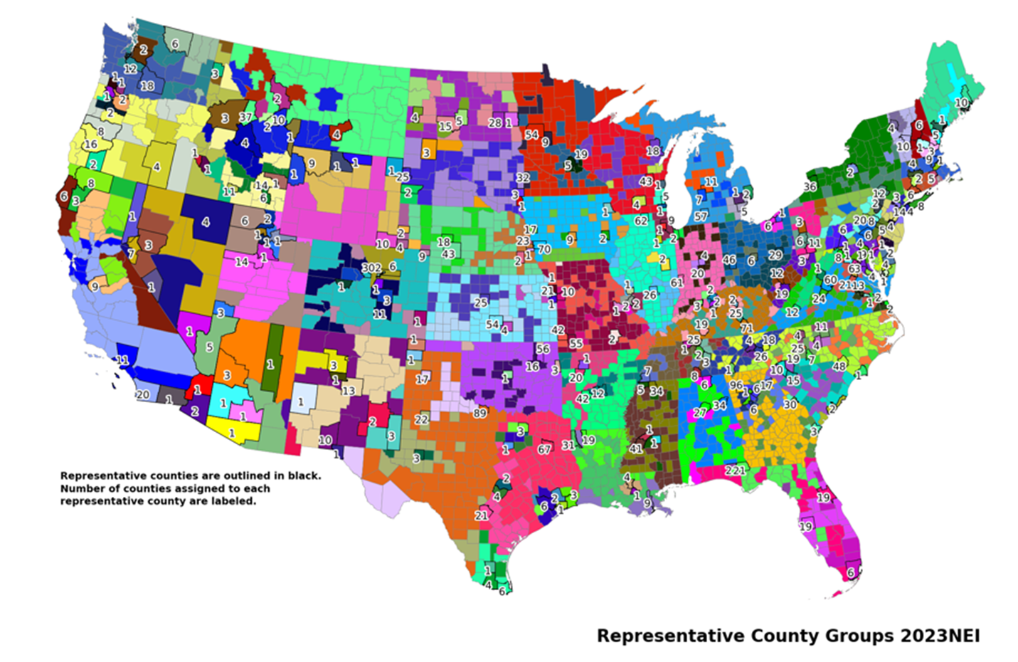
Figure 4.2: Representative County groups for the 2023 NEI

Download Figure

4.6.2.2 Fuel Months

A “fuel month” indicates when a particular set of fuel properties should be used in a MOVES simulation. Similar to the representative county, the fuel month reduces the computational time of MOVES by using a single month to represent a set of months during which a specific fuel has been used in a representative county. Because there are winter fuels and summer fuels, EPA used January to represent October through April and July to represent May through September. For example, if the grams/mile exhaust emission rates in January are identical to February’s rates for a given representative county, and temperature (as well as other factors), then we use a single fuel month to represent January and February. In other words, only one of the months needs to be modeled through MOVES to obtain the necessary emission factors. The hour-specific VMT, temperature and other factors for February are still used to calculate emissions in February, but the emission factors themselves do not need to be created, since one month can sufficiently represent the other month. The fuel months used for each representative county are provided in the MFMREF file in the supplementary materials (see Table 4.17 for access information).

4.6.2.3 Fuels

For the 2023 NEI, fuel property information came from the MOVES5 default database movesdb20241112. The fuels information was derived from retail survey data. For a national inventory such as the NEI, this approach provides a more consistent and comprehensive result with respect to fuel use and fuel impacts on emission rates. More details on development of the MOVES fuel supply is available in this MOVES technical support document: Fuel Supply Defaults: Regional Fuels and the Fuel Wizard in MOVES3.

For 2023 the nationwide fuel supply assumed 100% market share E10 ethanol blends in gasoline except for Alaska which assumes E0. All diesel was assumed to be 6 ppm sulfur, and onroad diesel was 100% market share B5 biodiesel blends nationwide.

4.6.3 Temperature and humidity

Ambient temperature can have a large impact on emissions. Low temperatures are associated with high start emissions for many pollutants. High temperatures and high relative humidity are associated with greater running emissions due to the increase in the heat index and resulting higher engine load for air conditioning. High temperatures also are associated with higher evaporative emissions.

The 12-km gridded meteorological input data for the entire year of 2023 covering the continental U.S. were derived from simulations of version 4.4.2 of the Weather Research and Forecasting Model (WRF), Advanced Research WRF core [ref 1]. The WRF Model is a mesoscale numerical weather prediction system developed for both operational forecasting and atmospheric research applications. The Meteorology-Chemistry Interface Processor (MCIP) [ref 2] was used as the software for maintaining dynamic consistency between the meteorological model, the emissions model, and air quality chemistry model.

EPA applied the SMOKE program Met4moves [ref 3] to the gridded, hourly meteorological data (output from MCIP) to generate a list of the maximum temperature ranges, average relative humidity, and temperature profiles that are needed for MOVES to create the emission-factor lookup tables. “Temperature profiles” are arrays of 24 temperatures that describe how temperatures change over a day, and they are used by MOVES to estimate vapor venting emissions. The hourly gridded meteorological data (output from MCIP) was also used directly by SMOKE (see Section 4.6.9).

The temperature lists were organized based on the representative counties and fuel months as described in Section 4.6.2. Temperatures were analyzed for all the counties that are mapped to the representative counties, i.e., for the county groups, and for all the months that were mapped to the fuel months. EPA used Met4moves to determine the minimum and maximum temperatures in a county group for the January fuel month and for the July fuel month, and the minimum and maximum temperatures for each hour of the day. Met4moves also generated temperature profiles using the minimum and maximum temperatures and 5 °F intervals. In addition to the meteorological data, the representative counties and the fuel months, Met4moves uses spatial surrogates to determine which grid cells from the meteorological data have roads and uses the WRF temperature and relative humidity data from those areas. For example, if a county had a mountainous area with no roads, the grid cells with no roads would be excluded from the meteorological processing. The spatial surrogates used for the 2023 NEI were based on activity data such as annual average daily traffic from the Highway Performance Monitoring System (HPMS) for the year 2022, as well as NLCD land use for the year 2019, with the goal of better characterizing the spatial variability of the onroad mobile source emissions.

For the 2023 NEI, MOVES was run with the a copy of the public MOVES5 default database movesdb20241112_nonoxadj (part of MOVES_Input_DBs.zip in Table 4.17) to prevent the model from making adjustments to NOx based on humidity levels. Instead, gridded hourly humidity values are used in SMOKE-MOVES to compute NOx adjustments to the unadjusted emissions output from MOVES.

Met4moves computes the range of temperatures needed by each representative county for each fuel month (i.e., 5-month summer season or 7-month winter season). When the emission factors are applied by SMOKE, the appropriate temperature bin and fuel month are used to compute the emissions. EPA used a 5 °F temperature bin size for RatePerDistance (RPD), RatePerVehicle (RPV), RatePerHour (RPH), RatePerHourONI (RPHO), and RatePerStart (RPS).

Met4moves can be run in daily or monthly mode for producing SMOKE input. In monthly mode, the temperature range is determined by looking at the range of temperatures over the whole month for that specific grid cell. Therefore, there is one temperature range per grid cell per month. While in daily mode, the temperature range is determined by evaluating the range of temperatures in that grid cell for each day. The output for the daily mode is one temperature range per grid cell per day and is a more detailed approach for modeling the vapor venting RatePerProfile (RPP) based emissions. EPA ran Met4moves in daily mode for the 2023 NEI. The temperature data output from Met4moves (2023NEI_RepCounty_Temperatures.zip) are provided with the supporting data in Table 4.17. The resulting temperatures for the representative counties are provided in the supplementary materials (see Table 4.17 for access information). The gridded, hourly temperature data used are publicly available only upon request and with provision of a disk media to copy these very large datasets.

4.6.4 VMT, vehicle population, speed, hoteling, starts, and ONI activity data

The activity data used to compute onroad mobile source emissions for the 2023 NEI uses EPA-computed data where state/local agencies did not provide their own data or where provided data did not pass quality assurance checks. These “default” (but county-specific) data were derived from Federal Highway Administration Data (FHWA) information including the published Highway Statistics 2023 [ref 4], along with county-level VMT data that is then allocated to vehicle type, fuel type, and road type. Some additional data sources were also used. The development of the default data is described in detail in 2023 NEI_default_onroad_activity_approach.pdf, which is listed with the supporting data in Table 4.17.

As discussed above, SMOKE combines the MOVES emission factors for each representative county with county-specific VMT, population, and hoteling data to compute the emissions for each individual county. These activity data are provided to SMOKE in a flat file format, and the source of the data varies according to area of the country and depending on whether the state/local agency submitted data for the 2023 NEI. The final activity data used are a combination of submitted data and EPA-developed data and are provided with the supporting data in (2023NEI_onroad_activity_final.zip).

For the counties for which an agency submitted a CDB (the dark blue areas shown previously in Figure 4.1), EPA ran scripts to extract the agency-submitted data from the CDBs and reformatted it into the flat file text file format that can be input to SMOKE (i.e., FF10). For the non-submitting areas of the U.S. (light blue areas in Figure 4.1), the EPA VMT, population, and hoteling were used. The 2023 default speeds are from the StreetLight telematics data. The CDBs use a distribution of speeds specific to hour, vehicle and road type, and weekday/weekend day types. SMOKE uses these same data, but the 16 speed bin distributions are averaged by hour, SCC, county, and weekday/weekend days. The FF10 creation scripts that read submitted CDBs are described separately by activity type below.

4.6.4.1 VMT FF10 file creation

The FF10-generation scripts read VMT flexibly from either the MOVES CDB table “sourceTypeYearVMT”, which contains annual VMT organized by MOVES source type, or “HPMSVtypeYear”, which contains annual VMT by groups of MOVES source types. The scripts disaggregate the VMT into fuel type, model year, and road type using a combination of other CDB tables as well as some MOVES default tables. First, the annual VMT is divided into model year using the CDB table with age distribution and the MOVES default database table containing relative annual mileage accumulation by age (“SourceTypeAge”). The scripts use these tables to create travel fractions for each source type and model year that sums to one (1) by source type.

Next, the VMT is further divided into fuel type categories of gasoline, diesel, CNG, E85, and electric vehicles – preferentially by using submitted MOVES CDB tables “AVFT” to determine the split of engine-fuel types by model year and “FuelUsageFraction” to determine the percent of flex-fuel engines that actually use E85. Flex-fuel engines refer to those capable of operating on either E85 or conventional gasoline, the percentage of which could be a function of local availability of the alternative fuel. Because the AVFT and FuelUsageFraction tables are optional tables in a MOVES CDB, they were not always populated in a submitted database. In cases where data were not provided, the FF10-generation scripts automatically default to MOVES national distributions of fuel types and/or E85 availability, using the “SampleVehiclePopulation” and “FuelUsageFraction” tables of the model default database to fill the missing data. It is worth noting that several states do not have any VMT (or vehicle population) associated with flex-fuel vehicles because they submitted data indicating either no flex-fuel vehicle population or zero E85 fuel supply in the CDB tables.

Finally, the FF10-generation scripts read the CDB table “RoadTypeDistribution” to further split VMT (by fuel type) into the four MOVES road types (urban and rural, restricted and unrestricted access). The scripts aggregate VMT across model years to the SCC level (i.e., MOVES source type, fuel type, and road type) and report annual and monthly VMT (using the “MonthVMTFraction” CDB table) for each SCC in each county into a consolidated list. Additional processing was performed to develop the final VMT data that includes both annual and monthly totals. First state-submitted monthly profiles were applied where they were available and valid (as obtained from the “MonthVMTFraction” table in the CDBs). Streetlight data were used elsewhere for all vehicle types except 62s, which were treated as flat monthly where state-submitted data were not used.

4.6.4.2 Population FF10 file creation

The FF10-generation script that creates the SMOKE vehicle population (i.e., VPOP) data operates similarly to the VMT script just described, except that the calculations do not use travel fractions to disaggregate population by model year. First, the script reads the CDB “SourceTypeYear” table, which contains 2023 population by MOVES source type and divides it into model years based on the submitted CDB “SourceTypeAgeDistribution” table. For each vehicle model year, the scripts apportion vehicle populations to fuel types using the submitted CDB tables “AVFT” and “FuelUsageFraction”, or, if no data were provided, uses the national default corresponding data tables described in Section 4.6.4.1.

The FF10 scripts then aggregate population from the model year level back up to the SCC level (MOVES source type and fuel type, and the road type 1). The CreateFF10 script and the Reverse FF10 script that pull activity data in and out of CDBs are included with the or_scripts_2023.zip file that is included with the supporting data described in Table 4.17.

After the vehicle population and VMT data were finalized, the population and VMT were compared by county and source type to look for inconsistencies between the two datasets. Specifically, counties and source types with an unreasonably high miles per year per-vehicle average (VMT divided by VPOP) were identified and addressed. For counties and source types with a VMT/VPOP ratio above the threshold in Table 4.14, the vehicle population was increased so that the new VMT/VPOP ratio would equal the maximum allowable ratio. The thresholds used were based on the 90th to 95th percentile of VMT/VPOP ratio for each source type. The vehicle populations were adjusted to produce reasonable VMT/VPOP ratios because MOVES can output unrealistic emission factors when the VMT/VPOP ratios are unreasonably high. EPA only needed to add VPOP for heavy-duty vehicles and motorcycles.

Table 4.14: Maximum allowable miles-per-year per-vehicle average by source type

MOVES source type	Source type description	Maximum VMT VPOP ratio miles per year
11	Motorcycle	7,500
21	Passenger Car	31,000
31	Passenger Truck	31,000
32	Light Commercial Truck	31,000
41	Other Bus	130,000
42	Transit Bus	90,000
43	School Bus	30,000
51	Refuse Truck	60,000
52	Single Unit Short-haul Truck	45,000
53	Single Unit Long-haul Truck	60,000
54	Motor Home	7,000
61	Combination Short-haul Truck	150,000
62	Combination Long-haul Truck	150,000

4.6.4.3 Speed FF10 file creation

SMOKE uses speed data for all counties to look up the appropriate VMT-based emission factors by speed bin and SCC. The FF10 “SPEED” input for SMOKE is one of two speed-related inputs; the other, described below, contains hourly speed distributions by SCC and county, separately for weekdays and weekends. The FF10 speed file for SMOKE contains a single daily average speed by SCC and county as an annual average.

Because the hourly speed distributions described in the next section cover all counties and SCCs, the FF10 “SPEED” input for SMOKE is not used as part of the emissions calculations. However, SMOKE still requires an FF10 SPEED file to exist, even if it is not used. Because of this, a new and complete FF10 SPEED file was not generated for 2023, and we instead used an older FF10 SPEED file in SMOKE processing.

4.6.4.4 Speed Distribution

The SPDIST file is generated by reformatting the MOVES ‘avgSpeedDistribution’ CDB table into a form that can be accepted by SMOKE. The speed distribution (SPDIST) input for SMOKE is optional. Out of the three possible ways to model vehicle speeds in SMOKE, SPDIST provides the highest resolution to best match vehicle activity with the lookup tables of emission factors, which for the running processes are listed by MOVES 16 speed bins. The SPDIST file lists the fraction of time in each hour spent in each of the 16 speed bins, for weekday and weekend day types, by county, source type, and road type. MOVES provides distinct emission factors for each of the 16 speed bins, and the SPDIST tells SMOKE-MOVES how to weight each of the speed bins when computing the total emissions. For example, if the SPDIST specifies 55% of time is spent in speed bin 8 and 45% of time is spent in speed bin 9 for a particular county, hour/day, and SCC, the emission factors for those two speed bins are weighted according to those ratios. The SMOKE-MOVES calculations also take unit conversions into account, as the SPDIST fractions are per unit time, while RPD emission factors are per unit distance.

Speed data from the StreetLight dataset were used to generate hourly speed profiles by county, SCC, and month. The StreetLight data were converted into SMOKE format, gapfilled so that all counties and SCCs were covered, and modified as needed based on quality assurance checks. To cover gaps in speed distributions (missing hours on low-data-coverage road types in certain counties) EPA grouped across urban and rural roads within the county for a given roadway “access” type but never combining speed information to mix restricted (e.g., highways) with unrestricted (e.g., arterials and local roads).

During quality assurance review of the grouped speed profiles, it was apparent that the speeds were sometimes too different between urban and rural roads within the same county. Instead of urban/rural grouping in these cases, data were substituted from adjacent months for the same MOVES road type and county. For example, if December data on rural restricted roads in a county was lacking, the November data for rural restricted roads were sometimes a better match than December urban+rural restricted roads. The judgement of what grouping decision was the “better match” was informed from review of average hourly speed profiles for all twelve months on a single plot, with separate plots for each road type and county. EPA substituted months of speed profiles as needed. This month substitution logic was only applied to speed distributions. VMT fractions are allowed to go to zero (0) for some hours in low-data situations, while speed data may not be zero from a modeling standpoint.

4.6.4.5 Hoteling FF10 file creation

Hoteling activity refers to the time spent idling in a diesel long-haul combination truck during federally- mandated rest periods for long-haul trips. Drivers may spend these rest periods with the main engine on, a smaller auxiliary power unit (APU) engine on, plugged into an electric source if available, or simply leave the engine off. MOVES tracks the emissions from hoteling using the main engine idling versus those from APUs separately. SMOKE reads each type of hoteling hours by SCC and matches them to the appropriate MOVES emission factor from the `RatePerHour’ lookup table.

Submitting agencies have the option to directly provide MOVES with the number of hoteling hours (via the ‘hotellingHours’ table) and the percent of trucks by model year that use APUs (the ‘hotellingActivityDistribution’ table). These CDB tables are optional. When they are present, the FF10-generation scripts read them and translate them into the FF10 formats for SMOKE. If they are empty, the FF10-generation scripts calculate the hoteling consistently with the methodology used internally to MOVES. Thus, the scripts multiply the VMT for diesel-fueled long-haul combination truck VMT on restricted access roads (urban and rural together) with the national average rate of hoteling. For the 2023 NEI, the national average rate of hoteling was estimated by EPA to be 0.007248 hours per mile. The scripts use the submitted fractions of APU usage where available and rely on MOVES defaults otherwise.

For the 2023 NEI, EPA calculated all hoteling hours from the final VMT by SCC and county. These hoteling hours were inserted into the final set of “all CDBs” released with the modeling platform (see Section 4.8). The representative CDBs were not updated, nor do they need these data to generate hoteling emission factors. For the 2023 NEI, an adjustment to hoteling was made to address concerns raised by stakeholders about hoteling hours being artificially concentrated in areas with large amounts of combination truck VMT, but which were not necessarily areas that trucks stopped to take long rest breaks. This is particularly an issue in heavily traveled urban areas. The hoteling hours per county were compared to the number of truck stop spaces identified in the Shapefile on which the surrogate that spatially allocates hoteling emissions to grid cells is based. This Shapefile was created collaboratively with states during the development of the 2011 NEI and updated during subsequent NEI efforts. In the analysis, for each county, the maximum number of hoteling hours per year that could be supported by the number of specified parking spaces was computed using the formula:

max hours / year = number of spaces * 24 hours / day * 365 days / year

This assumes that all spaces are filled at all hours of the day. The maximum number of hours was subtracted from the number of hours assigned to that county to determine if the county was over-allocated with hoteling hours as compared to the known spots. For the remaining over-allocated counties, no analysis was performed and a factor to adjust the hoteling hours down to match the max hours per year for each county was computed and applied, although it was assumed that any county can support a minimum of 105,120 hoteling hours (i.e., 12 spaces’ worth). No adjustments to hoteling hours were made in counties for which hoteling hours were substantially under-allocated as compared to the number of available spots. Ideally, hoteling hours would be properly allocated to counties by someone familiar with traffic patterns in the local area.

4.6.4.6 Off-network idling hours FF10 file creation

After creating VMT inputs for SMOKE-MOVES, additional work needs to be done to generation Off-network idle (ONI) activity. ONI is defined in MOVES as time during which a vehicle engine is running idle and the vehicle is somewhere other than on the road, such as in a parking lot, a driveway, or at the side of the road. This engine activity contributes to total mobile source emissions but does not take place on the road network. Examples of ONI activity include:

• light duty passenger vehicles idling while waiting to pick up children at school or to pick up passengers at the airport or train station,
• single unit and combination trucks idling while loading or unloading cargo or making deliveries, and
• vehicles idling at drive-through restaurants.

Note that ONI does not include idling that occurs on the road, such as idling at traffic signals, stop signs, and in traffic—these emissions are included as part of the running and crankcase running exhaust processes on the other road types. ONI also does not include long-duration idling by long-haul combination trucks (hoteling/extended idle), as that type of long duration idling is accounted for in other MOVES processes. ONI activity is calculated based on VMT. For each representative county, the ratio of ONI hours to onroad VMT (on all road types) is calculated using the MOVES ONI Tool by source type, fuel type, and month. These ratios are then multiplied by each county’s total VMT (aggregated by source type, fuel type, and month) to develop the ONI activity data.

4.6.4.7 Starts FF10 file creation

The NEI accounts for start emissions separately from running emissions because the quantity and profile of the pollutants that vehicle engines generate are significantly different than when the running engine is fully warm. SMOKE uses the number of starts activity for all counties by SCC and matches it with the appropriate MOVES emission factor from the “RatePerStart” lookup table. The SMOKE FF10 file contains both an annual total and monthly values for the number of starts. EPA estimated the annual total starts by running MOVES in inventory mode at the county scale for all counties using vehicle population, age distribution, and fuel type mix consistent with the VPOP FF10 file for SMOKE. The MOVES run specification files to generate starts activity outputs included only Total Energy Consumption in the pollutant list for runtime efficiency.

4.6.5 Public release of the NEI county databases

Two sets of 2023 CDBs are available for download: (1) seeded CDBs, which have been altered to produce emission rates for all sources, roads and processes to account for represented counties that may have different distributions than their representative county, and (2) unseeded CDBs intended to be used with MOVES Inventory mode calculations. The unseeded CDBs are available for all U.S. counties, but the seeded CDBs are only available for the representative counties. See Table 4.17 for access details.

4.6.6 Seeded CDBs

The seeded county databases can be used with MOVES to generate emission factor lookup tables for SMOKE-MOVES. In order to create representative county CDBs for MOVES runs for SMOKE-MOVES modeling, EPA performed a “seeding” step, whereby values of zero (0) were updated to a small value of 1e-15. This seeding ensures that the lookup tables will be fully populated regardless of whether the representative county itself included activity for all of the categories covered. Seeding is necessary because counties mapping to the representative county may require an emission factor that would otherwise be missing. Note that the seeded CDBs each contain activity data for all of the counties represented by the CDB, not for a single county. The scripts used to develop the seeded CDBs are included in the or_scripts_2023.zip file described in Table 4.17.

4.6.7 Unseeded CDBs

In contrast to the seeded CDBs, the unseeded CDBs do not have any seeding performed on them and include activity data only for the individual county. This set of CDBs is true to the local conditions and could be used for MOVES inventory mode runs. The unseeded CDBs merge the databases that were agency-submitted with the default CDBs for 2023 that include updates based on FHWA, MOVES5, SPGM, and StreetLight telematics data. The unseeded CDB tables “SourceTypeYearVMT”, “SourceTypeYear”, “HotellingHoursPerDay”, and “HotellingActivityDistribution”, “monthVMTFraction”, “idleMonthAdjust”, and “startsMonthAdjust” are consistent with the SMOKE-ready files of 2023 VMT, population, hoteling, ONI, and starts. Because totals of ONI and starts in the SMOKE-ready files relied on MOVES5 defaults, the totals were not put back into the unseeded set of all CDBs; only their monthly variation was put into “idleMonthAdjust” for ONI and “startsMonthAdjust” for starts, because these relied on 2023 specific VMT data by month. Activity data can be taken in and out of the unseeded individual county CDBs using the CreateFF10 and ReverseFF10 scripts included in the or_scripts_2023.zip file described in Table 4.17.

4.6.8 Run MOVES to create emission factors

EPA ran MOVES for each representative county using January fuels and July fuels for the range of temperatures spanned by the represented county group and set of months associated with each fuel set (January and July). A runspec generator script created a series of runspecs (MOVES jobs) based on the outputs from Met4moves temperature information for all months of the year. Specifically, the script used a 5-degree temperature bin with the minimum and maximum temperature ranges from Met4moves and used the idealized diurnal profiles from Met4moves to generate a series of MOVES runs that captured the full range of temperatures for the county group for the months assigned to each fuel. The MOVES runs resulted in six emission factor tables for each representative county and fuel month: rate per distance (RPD), rate per vehicle (RPV), rate per hour (RPH), rate per profile (RPP), rate per start (RPS), and rate per hour for ONI (RPHO). After the MOVES runs completed, the post-processor script Moves2smk converted the MySQL tables into emission factor (EF) files that can be read by SMOKE. For more details on Moves2smk, see the SMOKE documentation [ref 5]. The post-processor scripts are available in 2023nei_or_postprocessing_jars.zip as described in Table 4.17.

4.6.9 Run SMOKE to create emissions

To prepare the NEI emissions, EPA first generated emissions at an hourly resolution using more detailed SCCs than are found in the NEI (i.e., by road type and aggregate processes). The SMOKE-MOVES program Movesmrg performs this function by combining activity data, meteorological data, and emission factors to produce gridded, hourly emissions. EPA ran Movesmrg for each of the sets of emission factor tables (RPD, RPV, RPH, RPP, RPS, and RPHO). During the Movesmrg run, the program used the hourly, gridded temperature (for RPD, RPV, RPH, RPS, and RPHO) or daily, gridded temperature profile (for RPP) to select the proper emissions rates and compute emissions. These calculations were done for all counties and SCCs in the SMOKE inputs, covering the continental U.S., as well as separate runs covering outlying areas (e.g., Alaska and Hawaii).

The emission processes in RPD model the on-roadway driving emissions. This includes the following emission processes: vehicle exhaust, evaporation, evaporative permeation, refueling, brake wear, and tire wear. For RPD, the activity data is monthly VMT, monthly speed (i.e., SMOKE variable of SPEED), and hourly speed distributions (i.e., SPDIST in SMOKE). The SMOKE program Temporal takes temporal profiles specific to vehicle type and road type and distributes the monthly VMT to day of the week and hour. Movesmrg reads the speed distribution data for that county and SCC and the temperature from the gridded hourly (MCIP) data and uses these values to look-up the appropriate emission factors (EFs) from the representative county’s EF table. It then multiplies this EF by temporalized and gridded VMT for that SCC to calculate the emissions for that grid cell and hour. This is repeated for each pollutant and SCC in that grid cell. The default diurnal and weekly VMT temporal profiles are based on StreetLight telematics data.

The emission processes in RPV model the parked or “off-network” emissions other than exhaust emissions from vehicle starts. This includes evaporative and evaporative permeation emission processes. For RPV, the activity data is vehicle population (VPOP). Movesmrg reads the temperature from the gridded hourly data and uses the temperature plus SCC and the hour of the day to look up the appropriate EF from the representative county’s EF table. It then multiplies this EF by the gridded VPOP for that SCC to calculate the emissions for that grid cell and hour. This repeats for each pollutant and SCC in that grid cell.

The emission processes in RPH model the parked emissions for combination long-haul trucks (source type 62) that are hoteling. This includes the following modes: extended idle and APUs. For RPH, the activity data is monthly hoteling hours. The SMOKE program Temporal takes a temporal profile and distributes the monthly hoteling hours to day of the week and hour. Movesmrg reads the temperature from the gridded hourly (MCIP) data and uses these values to look-up the appropriate emission factors from the representative county’s EF table. It then multiplies this EF by temporalized and gridded HOTELING hours for that SCC to calculate the emissions for that grid cell and hour. This is repeated for each pollutant and SCC in that grid cell.

The emission processes in RPP model the parked emissions for vehicles that are key-off. This includes the mode vehicle evaporative (fuel vapor venting). For RPP, the activity data is VPOP. Movesmrg reads the gridded diurnal temperature range (Met4moves’ output for SMOKE). It uses this temperature range to determine a similar idealized diurnal profile from the EF table using the temperature min and max, SCC, and hour of the day. It then multiplies this EF by the gridded VPOP for that SCC to calculate the emissions for that grid cell and hour. This repeats for each pollutant and SCC in that grid cell.

The rate per start (RPS) emissions include start exhaust and crankcase start exhaust emissions. SMOKE used RPS emission factors (ignoring the duplicate starts information from the RPV table) and combines the RPS factors with STARTS activity by county and SCC. The rate-per-hour-off network idling (RPHO) represents emissions that occur idling during deliveries and the pick-up and drop-off of passengers. SMOKE used RPHO emission factors combined with off-network idle (ONI) activity by county and SCC. The result of the Movesmrg processing is hourly data as well as daily reports for each of the processing streams (RPD, RPV, RPH, RPP, RPS, and RPHO). The results include emissions for every county in the continental U.S.

4.6.9.1 Spatial Surrogates

For the onroad sector, the on-network (RPD) emissions were spatially allocated differently from other off-network processes (e.g., RPV, RPP, RPHO). Surrogates for on-network processes are based on AADT data and off network processes (including the off-network idling included in RPHO) are based on land use surrogates as shown in Table 4.15. Emissions from the extended (i.e., overnight) idling of trucks were assigned to surrogate 205, which is based on locations of overnight truck parking spaces. The total of the gridded emissions for each county and hour are summed to develop the NEI.

Table 4.15: Off-network Mobile Source Surrogates

Source type	Source Type name	Surrogate ID	Description
11	Motorcycle	307	NLCD All Development
21	Passenger Car	307	NLCD All Development
31	Passenger Truck	307	NLCD All Development
32	Light Commercial Truck	308	NLCD Low + Med + High
41	Other Bus	306	NLCD Med + High
42	Transit Bus	259	Transit Bus Terminals
43	School Bus	508	Public Schools
51	Refuse Truck	306	NLCD Med + High
52	Single Unit Short-haul Truck	306	NLCD Med + High
53	Single Unit Long-haul Truck	306	NLCD Med + High
54	Motor Home	304	NLCD Open + Low
61	Combination Short-haul Truck	306	NLCD Med + High
62	Combination Long-haul Truck	306	NLCD Med + High

4.6.10 Post-processing to create an annual inventory

For the purposes of the NEI, EPA needed emissions data by county, SCC, and pollutant. EPA ran SMOKE-MOVES at a more detailed level including road type and emission processes (e.g., extended idle) and summed over road types and processes to create the more aggregate NEI SCCs. EPA developed and used a set of scripts to combine the emissions from the six sets of reports and from all days to create the annual inventory. The post processing scripts are named aq_cb6_saprc_20250821 and multipoll_20250821. They are available in the documentation (see Section 4.8. Emissions for the older Connecticut counties were reallocated to the new county equivalents using county-to-county translation factors supplied by Connecticut DEEP. For example, emissions from Fairfield County (09001) were translated to the three new county equivalents which overlap Fairfield County: Greater Bridgeport (09120), Naugatuck Valley (09140), and Western Connecticut (09190). VMT activity by town and by road type was used to calculate the reallocation factors. Road-type-specific county translation factors were applied to RPD emissions; translation factors specific to restricted highways were applied to RPH emissions; and non-road-type-specific translation factors were applied to other emission rates (RPP, RPV, RPS, and RPHO).

Five speciated PM2.5 pollutants (i.e., PEC, POC, PNO3, PSO4, and PMFINE) were added to the NEI data for summary purposes. Note that air quality modeling uses a finer breakdown of these pollutants. DIESEL-PM10 and DIESEL-PM25 were also added by copying the PM10 and PM2.5 pollutants (respectively) as DIESEL-PM pollutants for all diesel SCCs. See Section 4.6.1 for more details.